This post describes a simple method of reading resistive and capacitive sensors using a standard PC sound card. Virtually any desktop or laptop could be turned into a simple data acquisition system using this method. Thanks to moderate system requirements, even the very old computers can be repurposed for this application. Socket 478 based platforms from early 2000’s with integrated sound cards are readily available for ~free from recycling bins and are perfectly capable of running the data acquisition software (thankfully, Debian still supports 32-bit platforms). With the total cost of other components under $1, this can hopefully bring affordable and interactive data acquisition to DIYers, experimenters and students in science and physics classes. I do not recommend (in fact, I highly discourage) using this method for anything but educational purposes. It is not meant to be used for industrial or even lab data acquisition – there are much better alternatives.

Another point of this post is to demonstrate that old PC motherboards are under-appreciated in DIY circles. Even the older ATX motherboards are equipped with many useful capabilities:

• audio ADCs and DACs (AC-coupled)
• DC voltage DACs for fan speed control
• hall effect sensor encoders for fan RPM readback
• PWM outputs for RPM control on 4-pin fan headers
• I2C busses in video ports
• dry contact inputs: “chassis intrusion” switches, audio jack detection contacts on front panel audio headers
• multiple voltage references (~1V core and memory voltages, 3.3V, 5V, 12V)

In addition, newer motherboards are equipped with goodies like thermistor inputs (e.g. headers T_SEN1, T_SEN2, etc. on MSI motherboards) that might not necessarily measure temperatures of water cooling loops :)

Example circuits are purposefully simplified to utilize only widely available passive components. While the quality of signal processing can be improved by introducing simple buffering and amplification, additional opamps and voltage sources would unnecessarily complicate the method, introduce additional expenses, and require more advanced electronics and soldering skills to implement. Simplicity of using only passive networks is a desired feature, and not a bug.

The text, illustrations, schematics and code snippets of this post are provided “as-is” without warranty of any kind. Please refer to the LICENSE before using any of it.

The code is available on github.

TOC

• PC sound cards and audio interfaces
• Hardware and software
  • Sound card I/O
  • Sensors and passives
• Reading resistive sensors
  • Circuit design
  • Hardware setup
  • Software setup
  • Module description
  • Adjusting input gain
  • Temperature measurement
  • Measurement errors
• Reading capacitive or inductive sensors
  • Measuring frequency response
  • Capacitance or inductance measurements
  • Circuit design
  • Hardware setup
  • Software setup
  • Water level measurement
• Troubleshooting

PC sound cards and audio interfaces

PC sound cards can be useful for projects that require kHz-rate analog inputs (see DIY oscilloscope). However they can’t be directly used for measuring DC signals since audio ADCs reject the DC component. Hence, the consensus is that sound cards are useless for reading any sensors, and DIY monitoring projects are usually based on ubiquitous Arduinos and Raspberry Pies.

However, the majority of sensors aren’t inherently DC. Standardized sensor interfaces use DC signals (0-5V, 0-10V, 4-20mA) due to simplicity of measuring and generating DC voltages and currents. Many underlying sensing elements are inherently resistive (thermistors, strain gauges in force and pressure transducers, potentiometers, light dependent resistors, etc.), capacitive (non-contact displacement sensors, proximity sensors, flow meters, level sensors, accelerometers, etc.) or inductive. The convention of reading sensors using DC signals is merely a convenience.

This post demonstrates the approach to reading such sensors using a PC sound card. A 10k thermistor and a DIY level probe are used in this example, but these methods can be extended to any resistive, capacitive and inductive measurements.

Hardware and software

The system is based on a standard PC with an integrated sound card. I use an old AM2 motherboard running Debian, but this should work on any modern Linux distribution. The only OS-dependent part is the interface for playing/recording wav files to/from the sound card using PulseAudio. This could be adapted to work with the Windows sound subsystem as well.

I conventionally use python with numpy, scipy and matplotlib to glue the pieces together.

Sound card I/O

There are a few ways to physically interface with the sound card:

• use audio pig tail cables plugged into 3.5mm audio jacks (could be salvaged from old speakers, headphones, etc.)
• use dupont style sockets plugged into motherboard audio headers (could be salvaged from old PC cases)
  • note: make sure to activate front panel audio ports by connecting SENSE_SEND to SENSE1_RETURN and SENSE2_RETURN pins when using HD Audio headers.

Sensors and passives

I use a standard 10kΩ NTC thermistor salvaged from a digital thermometer as an example of a resistive sensor. These thermistors can be found for less than a dollar apiece on amazon or ebay.

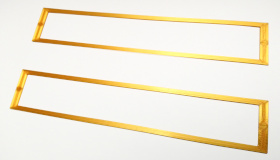
A level probe sensor is made from two pieces of aluminum foil (available from your kitchen drawers) glued onto plastic frames (can be 3d-printed or cut from a thin sheet of plastic – milk jug, old credit card, etc.).

Required passive components:

• three 10kΩ resistors for thermistor measurements
• one ~1mH inductor and one ~100nF capacitor for level probe measurements
  • note: different combinations of inductance and capacitance can be used as well (see Circuit design)

Reading resistive sensors

Circuit design

Resistance can be measured using an AC voltage source and AC voltmeter in a simple voltage divider arrangement:

The sound card output is used as the AC voltage source and its input is used as the voltmeter. A typical impedance of sound card outputs is under 0.1kΩ and it can be safely excluded from the equation. An input impedance is usually at the order of 10kΩ, so technically it should be considered for in resistance calculations. In practice, ignoring the input impedance results in errors of less than 1°C for the temperature range from -25°C to +25°C, and less than 2°C for temperatures below +35°C.

There is however one problem with this approach. Due to highly adjustable gain of audio DACs and ADCs (aka volume control), signal amplitudes cannot be easily converted to voltages and vice versa. E.g., audio output of my desktop has the RMS voltage around 1.2V at its max volume, but my laptop isn’t guaranteed to have the same voltage. In audio terms, this results in slight volume variations which isn’t a big deal. However these variations could introduce significant errors to resistance measurements.

We can of course measure the gain of audio input/output directly using a voltmeter. That would work, but such setup wouldn’t be portable since the measured gain would only describe the one particular system.

Another solution is to measure the ratio of input to output gains using a voltage divider with known resistors. This ratio can be used to determine the ratio of input to output voltages and calculate the unknown resistance. Thanks to the two available audio channels on stereo inputs and outputs, one channel can be used to determine the gain ratio and another one to measure the resistance.

Hardware setup

I used an audio breakout board with two 3.5mm ports to simplify the assembly:

Resistors R1, R2 and R3 are soldered directly on the board (R2 is in 0603 SMD package and is hard to see on the picture). Thermistor is connected to header pins. Input and output 3.5mm plugs are connected to the sound card using audio cables.

Software setup

NOTE: Make sure that both input and output jacks are plugged in before continuing. PulseAudio recognizes if ports are unplugged and deactivates them accordingly.

To communicate with the sound card, input and output devices must be identified. PulseAudio commands pacmd list-sinks and pacmd list-sources can be used to display available devices:

$ pacmd list-sinks | grep name:
    name: <alsa_output.pci-0000_00_07.0.analog-stereo>
$ pacmd list-sources | grep name: | grep -v monitor
    name: <alsa_input.pci-0000_00_07.0.analog-stereo>

In my case, the output device is alsa_output.pci-0000_00_07.0.analog-stereo and the input device is alsa_input.pci-0000_00_07.0.analog-stereo. These names should be specified in the $HOME/soundcard.cfg file in the following format (vol_record parameter is configured later):

[SOUNDCARD]
pa_sink = alsa_output.pci-0000_00_07.0.analog-stereo
pa_source = alsa_input.pci-0000_00_07.0.analog-stereo
vol_record = -1

Module description

All of the python glue is combined into a simple soundcard.py module with a handful of constants and functions.

Imports are as follows (numpy is used for array manipulation and scipy provides a convenient wavfile interface):

import configparser
import numpy as np
import os
import subprocess
import time
from scipy.io import wavfile

Constants specify the file locations, define the standard 44.1kHz PCM WAV format and time delays:

CFG_FILE = os.path.join(os.environ['HOME'], 'soundcard.cfg')
WAV_FILE_OUT = '/tmp/out.wav'
WAV_FILE_IN = '/tmp/in.wav'
SAMPLE_RATE = 44100
BIT_DEPTH = np.int16
WAV_FORMAT = 's16ne'
VOL_PLAY = 2 ** 16 - 1
DURATION_RECORD = 2
PAUSE_PRE_PLAY = 2
PAUSE_PRE_RECORD = 2
PAUSE_POST_RECORD = 2
DURATION_PLAY = DURATION_RECORD + PAUSE_PRE_RECORD + PAUSE_POST_RECORD

The config file is parsed and verifed using the configparser module:

config = configparser.ConfigParser()
config.read(CFG_FILE)
PA_SINK = config.get('SOUNDCARD', 'PA_SINK', fallback='')
PA_SOURCE = config.get('SOUNDCARD', 'PA_SOURCE', fallback='')
VOL_RECORD = config.getint('SOUNDCARD', 'VOL_RECORD', fallback=-1)
if PA_SINK == '' or PA_SOURCE == '' or VOL_RECORD == -1:
    config['SOUNDCARD'] = {'PA_SINK': PA_SINK, 'PA_SOURCE': PA_SOURCE, 'VOL_RECORD': VOL_RECORD}
    with open(CFG_FILE, 'w') as cfg:
        config.write(cfg)
if PA_SINK == '' or PA_SOURCE == '':
    raise ValueError(f'PA_SINK or PA_SOURCE are not set! Specify PulseAudio devices in {CFG_FILE}')

The following functions define the waveforms to be played over the audio output. A pure sine wave is an obvious choice, and a 440Hz (middle C) is a perfect pitch for the task. White noise is defined here as well – it is a useful test signal for frequency response measurements:

def sine_wave(frequency=440):
    time_points = np.linspace(0, DURATION_PLAY, SAMPLE_RATE * DURATION_PLAY)
    return np.iinfo(BIT_DEPTH).max * np.sin(frequency * 2 * np.pi * time_points)

def white_noise():
    return np.random.uniform(np.iinfo(BIT_DEPTH).min, np.iinfo(BIT_DEPTH).max, SAMPLE_RATE * DURATION_PLAY)

After playing this waveform through the sound card and recording it back, we need to make sure that the recorded sine wave isn’t clipped, otherwise the output amplitude won’t be determined correctly. This might happen if the recording level is too high. This function verifies that the waveform fits between the max and min values of 16-bit PCM WAV file:

def is_waveform_clipped(waveform):
    clipped_top = np.max(waveform) >= np.iinfo(BIT_DEPTH).max
    clipped_bottom = np.min(waveform) <= np.iinfo(BIT_DEPTH).min
    return clipped_top or clipped_bottom

The simplest way to play/record the waveforms to/from the sound card is to use paplay and parecord. These commands only work with wav files, so scipy.io.wavfile is used to convert the files to numpy arrays and vice versa. Prior to playing and recording the signal, input and output levels are adjusted to predefined levels using pacmd set-sink-volume and pacmd set-source-volume:

def write_waveform(waveform):
    if os.path.exists(WAV_FILE_OUT):
        os.remove(WAV_FILE_OUT)
    wavfile.write(WAV_FILE_OUT, SAMPLE_RATE, np.hstack((waveform, waveform)).astype(BIT_DEPTH))

def play_wav():
    subprocess.Popen(['pacmd', 'set-sink-volume', PA_SINK, '0'])
    subprocess.Popen(['pacmd', 'set-sink-volume', PA_SINK, f'{int(VOL_PLAY)}'])
    subprocess.Popen(['paplay', WAV_FILE_OUT, f'--device={PA_SINK}'])

def record_wav():
    if VOL_RECORD == -1:
        raise ValueError('VOL_RECORD parameter is not set! Use gain_tune.py to configure recording gain')
    if os.path.exists(WAV_FILE_IN):
        os.remove(WAV_FILE_IN)
    subprocess.Popen(['pacmd', 'set-source-volume', PA_SOURCE, '0'])
    subprocess.Popen(['pacmd', 'set-source-volume', PA_SOURCE, f'{int(VOL_RECORD)}'])
    subprocess.Popen(
        [
            'parecord',
            f'--device={PA_SOURCE}',
            f'--rate={SAMPLE_RATE}',
            f'--format={WAV_FORMAT}',
            '--channels=2',
            f'--process-time-msec={DURATION_RECORD*1000}',
            WAV_FILE_IN,
        ]
    )

def read_waveform():
    _, waveform = wavfile.read(WAV_FILE_IN)
    return waveform

Next function combines the following tasks:

• accept waveform numpy array parameter and save it to wav file
• start playing wav file to line output
• wait for output to stabilize
• start recording to wav file from line input
• wait while signal is being recorded
• stop recording process
• convert recorded wav file to numpy array
• wait for sound to finish playing and stop PulseAudio player
• verify that recorded waveform isn’t clipped

def play_and_record(waveform):
    write_waveform(waveform)
    time.sleep(PAUSE_PRE_PLAY)
    play_wav()
    time.sleep(PAUSE_PRE_RECORD)
    record_wav()
    time.sleep(DURATION_RECORD)
    subprocess.Popen(['pkill', 'parecord'])
    time.sleep(PAUSE_POST_RECORD)
    new_waveform = read_waveform()
    subprocess.Popen(['pkill', 'paplay'])
    if is_waveform_clipped(new_waveform):
        raise ValueError('Recorded waveform is clipped - reduce VOL_RECORD parameter')
    new_waveform_L = new_waveform.astype('int')[:, 0]
    new_waveform_R = new_waveform.astype('int')[:, 1]
    return new_waveform_L, new_waveform_R

Finally, a simple helper function is defined to calculate RMS values of waveforms:

def rms(waveform):
    return np.sqrt(np.mean(np.square(waveform)))

Adjusting input gain

To maximize the resolution of audio waveforms, recording levels should be adjusted in a way that scales input signal amplitudes close to the maximum range of 16-bit PCM WAV format. This is done by repeatedly playing and recording the sine wave while adjusting the recording level and testing the input for clipping. The gain_tune.py script tests multiple recording levels until it finds the highest one that doesn’t clip the signal. Recording level is then saved to the $HOME/soundcard.cfg config file:

import configparser
import numpy as np
import soundcard as sc
import subprocess
import time

MARGIN = 0.75
STEPS_TOTAL = 5

step = 0
lo, hi = 0, 65535
while True:
    vol_current = int((hi + lo) / 2)
    sc.VOL_RECORD = vol_current
    try:
        w_L, w_R = sc.play_and_record(sc.sine_wave())
        rms_L, rms_R = sc.rms(w_L), sc.rms(w_R)
        lo = vol_current
        step += 1
        print(f'no clipping detected at VOL_RECORD = {vol_current}, rms_L = {rms_L:.2f}, rms_R = {rms_R:.2f}')
    except ValueError:
        hi = vol_current
        print(f'clipping detected at VOL_RECORD = {vol_current}')
    if step > STEPS_TOTAL:
        vol_current = int(sc.VOL_RECORD * MARGIN)
        sc.config['SOUNDCARD']['VOL_RECORD'] = str(vol_current)
        with open(sc.CFG_FILE, 'w') as cfg:
            sc.config.write(cfg)
        print(f'VOL_RECORD value {vol_current} saved to {sc.CFG_FILE}')
        break

The level should also be adjusted for variabilities of input amplitude. In this case, they are caused by temperature variations. I use the thermistor to monitor outside temperatures: assuming high of 40°C on the worst summer day, the lowest corresponding resistance of 10kΩ thermistor is ~5kΩ. MARGIN is adjusted to reflect the voltage ratio of reference to measurement channels for this condition (adjust this margin accordingly for your sensors):

(10 kΩ / (10 kΩ + 10 kΩ)) / (10 kΩ / (5 kΩ + 10 kΩ)) = 0.75

The tuning script performs a binary search until the gain is determined with specified accuracy (determined by STEPS_TOTAL):

$ cat ~/soundcard.cfg | grep vol_record
vol_record = -1
$ python3 gain_tune.py
clipping detected at VOL_RECORD = 32767
no clipping detected at VOL_RECORD = 16383, rms_L = 5516.48, rms_R = 5291.19
no clipping detected at VOL_RECORD = 24575, rms_L = 18677.35, rms_R = 17995.21
clipping detected at VOL_RECORD = 28671
clipping detected at VOL_RECORD = 26623
no clipping detected at VOL_RECORD = 25599, rms_L = 21104.81, rms_R = 20477.67
no clipping detected at VOL_RECORD = 26111, rms_L = 22477.60, rms_R = 22008.95
clipping detected at VOL_RECORD = 26367
no clipping detected at VOL_RECORD = 26239, rms_L = 22470.11, rms_R = 22005.82
no clipping detected at VOL_RECORD = 26303, rms_L = 22469.06, rms_R = 22005.82
VOL_RECORD value 19727 saved to /home/nagimov/soundcard.cfg
$ cat ~/soundcard.cfg | grep vol_record
vol_record = 19727

Temperature measurement

Resistance values of R_1, R_2 and R_3 are measured directly and used in the thermistor.py script to slightly improve the accuracy. Steinhart-Hart equation is used for resistance-to-temperature conversion:

import numpy as np
import soundcard as sc

R_1 = 9.95e3
R_2 = 10.0e3
R_3 = 9.94e3
A = 2.108508173e-3
B = 0.7979204727e-4
C = 6.535076315e-7

while True:
    w_L, w_R = sc.play_and_record(sc.sine_wave())
    rms_L, rms_R = sc.rms(w_L), sc.rms(w_R)
    gain_ratio = rms_R * (R_1 + R_2) / R_2
    R_NTC = R_3 * (gain_ratio / rms_L - 1)
    T_NTC = 1 / (A + B * np.log(R_NTC) + C * np.log(R_NTC) ** 3) - 273.15
    print(f'R_NTC = {R_NTC:.1f} Ohm, T_NTC = {T_NTC:.1f} C')

Measurement errors

To simplify the measurement, impedance of the sound card input is not accounted for. Measurement errors caused by this are tolerable for the ambient temperature monitoring.

Estimated measurement errors in the range from 1kΩ to 100kΩ (defined using an Ohm-meter and an adjustable potentiometer):

Same measurement errors represented in temperature units in the range from -25°C to +35°C:

Errors caused by the unknown input impedance can be evaluated similarly for other kinds of measurements. These errors can be reduced by substracting the above error curves from measurements. Another method is to define the input impedance by measuring a known resistance and adjusting for the additional voltage drop at the input side.

Reading capacitive or inductive sensors

For resistance measurements, the AC signal from the sound card was fixed at 440Hz, since resistive circuits (i.e. without inductance and capacitance) are not affected by signal frequency. For circuits with capacitors or inductors this is not the case – their behavior is frequency dependent. This fact could be exploited to read such sensors by measuring their frequency response characteristics. Since sound cards can both generate and record AC signals at various frequencies, they can be used to measure capacitance and inductance. Note that the usable frequency range of audio equipment (including PC sound cards) is limited to the range of audible frequencies: from ~20Hz to ~20,000Hz. The exact low and high limits are hardware-dependent and can be determined experimentally.

Measuring frequency response

The frequency of output audio signal can be adjusted in the code by supplying an optional freq parameter to the sine_wave() function. To measure the frequency response characteristic of circuits, the output signal frequency is varied in steps within defined limits and the input amplitude is measured at each step.

In the first demonstration, the sound card itself is characterized for the frequency response. In this measurement, the output of the sound card is connected directly to its input using an audio cable. With no circuitry in between, this measurement describes the combined frequency response of the DAC and ADC circuits of the sound card.

The first step is to re-tune the recording gain using the gain_tune.py script:

$ python3 gain_tune.py
clipping detected at VOL_RECORD = 32767
no clipping detected at VOL_RECORD = 16383, rms_L = 11937.79, rms_R = 11494.02
clipping detected at VOL_RECORD = 24575
clipping detected at VOL_RECORD = 20479
no clipping detected at VOL_RECORD = 18431, rms_L = 17088.12, rms_R = 16542.01
no clipping detected at VOL_RECORD = 19455, rms_L = 20112.67, rms_R = 19555.55
no clipping detected at VOL_RECORD = 19967, rms_L = 21752.07, rms_R = 21287.34
no clipping detected at VOL_RECORD = 20223, rms_L = 22599.30, rms_R = 22116.54
no clipping detected at VOL_RECORD = 20351, rms_L = 23028.75, rms_R = 22536.46
VOL_RECORD value 15263 saved to /home/nagimov/soundcard.cfg

The measurement is done using the freq_sweep.py script:

import matplotlib.pyplot as plt
import numpy as np
import soundcard as sc

# frequency sweep
freq = np.geomspace(3, 20000, num=200)
with open(__file__.replace('.py', '.csv'), 'w') as csv:
    csv.write('freq, rms_L, rms_R\n')
    for f in freq:
        w_L, w_R = sc.play_and_record(sc.sine_wave(f))
        rms_L, rms_R = sc.rms(w_L), sc.rms(w_R)
        print(f'f = {f:.2f}, rms_L = {rms_L:.2f}, rms_R = {rms_R:.2f}')
        csv.write(f'{f:.2f}, {rms_L:.2f}, {rms_R:.2f}\n')
sweep = np.genfromtxt(__file__.replace('.py', '.csv'), delimiter=',', names=True)
# plot
plt.figure(figsize=(9, 2))
plt.plot(sweep['freq'], sweep['rms_L'], '.-', label='L ch', lw=0.5, ms=1)
plt.plot(sweep['freq'], sweep['rms_R'], '.-', label='R ch', lw=0.5, ms=1)
plt.tight_layout()
plt.legend(loc='upper left')
plt.xscale('log')
plt.savefig(__file__.replace('.py', '.png'), dpi=100)

The result of this measurement might look familiar – it is a typical frequency response curve of audio systems:

In my case, the response curve is approximately flat in the interval from 30Hz to 17,000Hz. Note that this range is hardware-dependent: higher-end audio chips produce “flatter” response, while my 10-years old motherboard is far from the ideal “20Hz to 20kHz” range. This curve also defines a usable range for frequency response measurements – at frequencies below 30Hz or above 17,000Hz the sound card itself introduces measurement errors. This could be somewhat mitigated by introducing correction factors that account for sound card characteristics, but the benefits are not worth the additional steps in this case.

Capacitance or inductance measurements

Now that the simple frequency response measurement is figured out, it could be extended to include the features required for capacitance or inductance measurements. Note that the example below uses a capacitive water level sensor with a fixed inductor, but the method can be adjusted for variable inductance sensors with fixed capacitors.

Circuit design

To read capacitance or inductance using frequency response curves, a measurement circuit must meet the following criteria:

• have an easily identifiable feature on its frequency characteristic
• directly correlate this feature to the capacitance or inductance of its component
• contain this feature within the usable frequency response range of the sound card

The simplest circuit made of entirely resistors and capacitors that exhibits such behavior is a passive band-pass filter:

When using identical resistors and capacitors on a low-pass and high-pass sides of the band-pass filter, the resulting frequency response peaks at its cut-off frequency:

f = 1 / (2 * π * R * C)

However it has a disadvantage – in order for peak to be “sharp” and easily identifiable, capacitors in the circuit must be identical. This complicates measurement of capacitive sensors, i.e. two identical sensors measuring the same parameter must be used with this circuit.

At a cost of somewhat increased complexity due to an additional inductor, RLC circuits exhibit similar behavior and utilize only one capacitor. There are many topologies to choose from. In this case, a series band-stop RLC filter is used:

The response curve of this filter has a “dip” around its center frequency (see below). With a known inductance in the circuit, capacitance can be correlated to the frequency of the peak (and vice-versa for inductive measurements):

f = 1 / (2 * π * sqrt(L * C))

Since the center frequency of RLC filters only depends on inductance and capacitance, knowledge of the reference gain is not required for frequency response measurements. This means that both audio channels can be used independently, allowing for simultaneous measurements of two capacitive or inductive sensors.

The inductor-capacitor combination must be chosen carefully to ensure that the center frequency of the band-stop filter can be accurately determined using the sound card. The usable frequency range of my sound card lies between 30Hz and 17,000Hz. In order to detect the peak on the frequency response characteristic, a few samples must be measured at frequencies below and above the peak. The corresponding center frequency of the band-stop filter should therefore be always higher than ~40Hz and lower than ~15,000Hz.

For capacitive measurements, constant inductances are used in the circuit. I salvaged my inductors from an old LED bulb, and they turned out to be 1.4mH and 3.3mH. Capacitance range that can be measured using 1.4mH inductor on my audio ADC is:

C_min = 1 / (4 * π^2 * (15,000 Hz)^2 * 1.4e-3 H) = 80.414 nF
C_max = 1 / (4 * π^2 * (40 Hz)^2 * 1.4e-3 H) = 11308 uF

Range for 3.3mH inductor:

C_min = 1 / (4 * π^2 * (15,000 Hz)^2 * 3.3e-3 H) = 34.115 nF
C_max = 1 / (4 * π^2 * (40 Hz)^2 * 3.3e-3 H) = 4797.4 uF

The capacitance of my DIY water level probe ranges from 0 to ~300nF. Since its lower bound is less than C_min, an additional capacitor must be added to offset the center frequency down to detectable ~15,000Hz and ensure that peaks on frequency characteristics are always detectable. Capacitors are selected by rounding up the values of C_min. In this case, a 100nF capacitor is added to a 1.4mH inductor and a 47nF capacitor is added to a 3.3 mH inductor. In this configuration, even the lowest capacitance of the sensor (i.e. at zero water level) produces frequency characteristics with a detectable peak:

1 / (2 * π * sqrt(100e-9 F * 1.4e-3 H)) = 13451 Hz
1 / (2 * π * sqrt(47e-9 F * 3.3e-3 H)) = 12778 Hz

For inductive sensors, similar calculations can be used for capacitor selection.

Finite input impedance of audio ADCs (in the order of 10kΩ) eliminates the need for an additional resistor. Audio output is used to excite the circuit at various frequencies and the response is recorded at the input side. To simplify the math, capacitive sensors are connected in parallel with fixed capacitors, so the total capacitance of RLC filters is the sum of the two. For inductance measurements, sensors would be connected in series with fixed inductors, when required.

Hardware setup

This simple stripboard allows quickly connecting the sensors and additional capacitors in parallel to the fixed capacitor via header pins and sockets:

Software setup

Center frequencies of RLC circuits on both channels are measured using freq_sweep_peak.py script:

import matplotlib.pyplot as plt
import numpy as np
import soundcard as sc

peak, argpeak = np.min, np.argmin  # replace with (np.max, np.argmax) for max values

# frequency sweep
freq = np.geomspace(30, 17000, num=100)
with open(__file__.replace('.py', '.csv'), 'w') as csv:
    csv.write('freq, rms_L, rms_R\n')
    for f in freq:
        w_L, w_R = sc.play_and_record(sc.sine_wave(f))
        rms_L, rms_R = sc.rms(w_L), sc.rms(w_R)
        print(f'f = {f:.2f} Hz, rms_L = {rms_L:.2f}, rms_R = {rms_R:.2f}')
        csv.write(f'{f:.2f}, {rms_L:.2f}, {rms_R:.2f}\n')
sweep = np.genfromtxt(__file__.replace('.py', '.csv'), delimiter=',', names=True)
freq_L_peak, rms_L_peak = sweep['freq'][argpeak(sweep['rms_L'])], peak(sweep['rms_L'])
freq_R_peak, rms_R_peak = sweep['freq'][argpeak(sweep['rms_R'])], peak(sweep['rms_R'])
# plot
plt.figure(figsize=(9, 2))
plt.plot(sweep['freq'], sweep['rms_L'], '.-', label=f'L ch: peak @ {freq_L_peak:.2f} Hz', lw=0.5, ms=1)
plt.plot(sweep['freq'], sweep['rms_R'], '.-', label=f'R ch: peak @ {freq_R_peak:.2f} Hz', lw=0.5, ms=1)
plt.plot([freq_L_peak, freq_R_peak], [rms_L_peak, rms_R_peak], '+', ms=7)
plt.tight_layout()
plt.legend(loc='lower left')
plt.xscale('log')
plt.savefig(__file__.replace('.py', '.png'), dpi=100)

The center frequencies are detected at close to the expected values (12778Hz and 13451Hz):

For the following plot, various capacitors are used to mock the sensor. Frequency response is measured for each capacitor on the left channel:

And on the right channel:

Note the differences between the channels:

• peaks are “sharper” and distributed further apart on the left channel, which improves the accuracy and resolution of detected peak frequencies
• frequency range occupied by the peaks is narrower on the right channel, which increases the range of capacitances that could be measured with a given sound card

This demonstrates that selection of inductors is a trade-off between measurement range and accuracy. The inductor affects both the absolute value of the center frequency (f) and the bandwidth of the filter (Δf):

f = 1 / (2 * π * sqrt(L * C))
Δf = R / (2 * π * L)

Given a constant resistance R and capacitance C, higher inductance L will reduce the bandwidth of the filter (i.e. make the peaks “sharper”) at a cost of reduced sensitivity of the filter to changing capacitance C.

While reliably detecting the center frequency of the band-pass filter, the high-resolution frequency sweep requires a large number of measurements, and therefore takes a long time to complete. To reduce the measurement time, freq_iter_peak.py script can be used. It employs a simple iterative optimization to find the peaks faster:

import matplotlib.pyplot as plt
import numpy as np
import soundcard as sc

STEPS = 4
ITERS = 4

peak, argpeak = np.min, np.argmin  # replace with (np.max, np.argmax) for max values

# optimization
freq = {'L': np.geomspace(30, 17000, num=STEPS).tolist(), 'R': np.geomspace(30, 17000, num=STEPS).tolist()}
rms = {'L': [], 'R': []}
for n, ch in [(0, 'L'), (1, 'R')]:
    print(f'Optimizing channel {ch}')
    for f in freq[ch]:
        w = sc.play_and_record(sc.sine_wave(f))
        rms[ch].append(sc.rms(w[n]))
        print(f'f = {f:.2f} Hz, rms_{ch} = {rms[ch][-1]:.2f}')
    for i in range(ITERS):
        peak_indices = np.argwhere(rms[ch] == peak(rms[ch])).flatten()
        peak_index_left, peak_index_right = max(0, min(peak_indices) - 1), min(max(peak_indices) + 1, len(freq[ch]) - 1)
        print(f'{" "*4*i}refining peak: f_{ch} = {freq[ch][peak_indices[0]]:.2f} Hz, peak_{ch} = {peak(rms[ch]):.2f}')
        freq_fine = np.geomspace(freq[ch][peak_index_left], freq[ch][peak_index_right], num=STEPS + 2)
        freq_fine = [k for k in freq_fine[1:-1] if k not in freq[ch]]  # don't duplicate measurements
        for f in freq_fine:
            freq_pos = np.argwhere(f < np.array(freq[ch])).flatten()[0]
            w = sc.play_and_record(sc.sine_wave(f))
            rms[ch].insert(freq_pos, sc.rms(w[n]))
            freq[ch].insert(freq_pos, f)
            print(f'{" "*4*(i+1)}f = {f:.2f} Hz, rms_{ch} = {rms[ch][freq_pos]:.2f}')
    peak_indices = np.argwhere(rms[ch] == peak(rms[ch])).flatten()
    peak_freq = freq[ch][peak_indices[len(peak_indices) // 2]]
    print(f'{"    "*ITERS}final peak: f_{ch} = {peak_freq:.2f} Hz, rms_{ch} = {peak(rms[ch]):.2f}')
    freq[f'{ch}_peak'], rms[f'{ch}_peak'] = freq[ch][argpeak(rms[ch])], peak(rms[ch])
# plot
plt.figure(figsize=(9, 2))
for ch in ['L', 'R']:
    plt.plot(freq[ch], rms[ch], '.-', label=f'{ch} ch: peak @ {freq[f"{ch}_peak"]:.2f} Hz', lw=0.5, ms=3)
    plt.plot(freq[f'{ch}_peak'], rms[f'{ch}_peak'], '+', ms=7)
plt.tight_layout()
plt.legend(loc='lower left')
plt.xscale('log')
plt.savefig(__file__.replace('.py', '.png'), dpi=100)

Off-topic note: reducing the number of measurements required to find the center frequencies of RLC-circuits is a typical example of mathematical optimization. The iterative approach described above utilizes the simplest Greedy algorithm to find the local minimum of the frequency characteristic. More complicated optimization algorithms (e.g. Gradient descent) can be employed to reduce the measurement time even further.

This graph demonstrates why it is both faster and more accurate. Since measurements are only taken around “important” regions of interest, every consecutive measurement further improves the accuracy:

Can we do any faster? Yes! The freq_fft_peak.py script can be used to excite the circuit with white noise and measure the frequency response at the output in a single measurement using a Fast Fourier Transform. While the theory behind this method is heavy on math, the implementation is very simple thanks to the python libraries:

import matplotlib.pyplot as plt
import numpy as np
import soundcard as sc

peak, argpeak = np.min, np.argmin  # replace with (np.max, np.argmax) for max values

# fft peak
freq_bins = np.geomspace(30, 17000, 300)
freq_bins_cent = [np.mean([lo, hi]) for lo, hi in zip(freq_bins[:-1], freq_bins[1:])]
w_L, w_R = sc.play_and_record(sc.white_noise())
freq = np.fft.rfftfreq(len(w_L), 1 / sc.SAMPLE_RATE)
fft_L, fft_R = np.abs(np.fft.rfft(w_L)), np.abs(np.fft.rfft(w_R))
fft_L_bins = [np.mean(fft_L[np.where((freq > lo) & (freq <= hi))]) for lo, hi in zip(freq_bins[:-1], freq_bins[1:])]
fft_R_bins = [np.mean(fft_R[np.where((freq > lo) & (freq <= hi))]) for lo, hi in zip(freq_bins[:-1], freq_bins[1:])]
freq_L_peak, fft_L_peak = freq_bins_cent[argpeak(fft_L_bins)], peak(fft_L_bins)
freq_R_peak, fft_R_peak = freq_bins_cent[argpeak(fft_R_bins)], peak(fft_R_bins)
# plot
scale = 0.01
plt.figure(figsize=(9, 2))
plt.plot(freq_bins_cent, np.array(fft_L_bins)*scale, '.-', label=f'L ch: peak @ {freq_L_peak:.2f} Hz', lw=0.5, ms=1)
plt.plot(freq_bins_cent, np.array(fft_R_bins)*scale, '.-', label=f'R ch: peak @ {freq_R_peak:.2f} Hz', lw=0.5, ms=1)
plt.plot([freq_L_peak, freq_R_peak], [fft_L_peak*scale, fft_R_peak*scale], '+', ms=7)
plt.tight_layout()
plt.legend(loc='lower left')
plt.xscale('log')
plt.savefig(__file__.replace('.py', '.png'), dpi=100)

As a result, the entire frequency range is analyzed in a single measurement. Note that the peaks are consistent with values from the iterative optimization plot:

The last step is to back-calculate the capacitance from the frequency response. The above two charts are taken using a 470nF capacitor on the left channel and a 47nF capacitor on the right channel. Measurements are within ±10% of expected values:

C_L = 1 / (4 * π^2 * (3,800 Hz)^2 * 3.3e-3 H) - 47e-9 F = 484 nF
C_R = 1 / (4 * π^2 * (11,200 Hz)^2 * 1.4e-3 H) - 100e-9 F = 44.2 nF

Water level measurement

A useful example of a capacitive sensor is a liquid level probe. The sensor can be easily made from two pieces of aluminum foil, affixed close to each other without touching anywhere. I used two 3d-printed plastic frames to hold two strips of foil using super-glue, and attached a piece of jumper wire onto each strip:

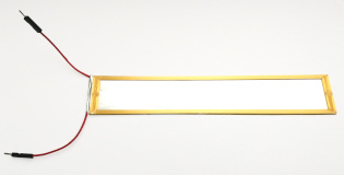
When the water level goes up it fills a portion of the gap between the wires. Since the relative permittivity of water is ~80 times higher than that of air, the total capacitance of the sensor increases. This change in capacitance can be detected and translated to a liquid level:

Troubleshooting

• Depending on the setup (PC configuration, current CPU load, etc.), OS “reaction time” can vary. Sometimes it takes a second or two for PulseAudio to play the wave file, there is another delay for the recording process to “catch up”, etc. To achieve consistent measurements, delays are introduced into the playing and recording sequence. If used on an outdated hardware, timing variables (DURATION_RECORD, PAUSE_PRE_PLAY, PAUSE_PRE_RECORD, PAUSE_POST_RECORD, and DURATION_PLAY) might need to be increased in the soundcard.py module. Alternatively, when used on a fast modern PC, these variables can be decreased to speed up the measurements.
• Whenever PulseAudio errors are displayed (e.g. Stream error: No such entity or No sink/source found by this name or index), make sure that correct PulseAudio source and sink are specified in the soundcard.cfg file.